1 글꼴 분류¹

활자(Type)는 본래는 글자를 만드는 데 사용된 나무 또는 금속 조각을 일컫는 말이었습니다.
타이포그래피(Typography): 인쇄된 텍스트의 스타일과 모양을 가리키는 디자인 용어입니다.
서체(또는 글꼴 모음, Typeface): 글자 및 기호가 서로 비슷한 특징을 가지도록 디자인된 문자fh 타임즈(Times), 에어리얼(Arial) 및 미니언(Minion)을 들 수 있습니다.
글꼴(Font): 서체의 특정 스타일을 지칭하는데, 예를 들어, 에어리얼 블랙(Arial Black)은 에어리얼 서체 중 한 글꼴이며, 미니언 프로 이탤릭체(Minion Pro Italic)는 미니언 글꼴 모음에 포함되어 있는 글꼴이다.

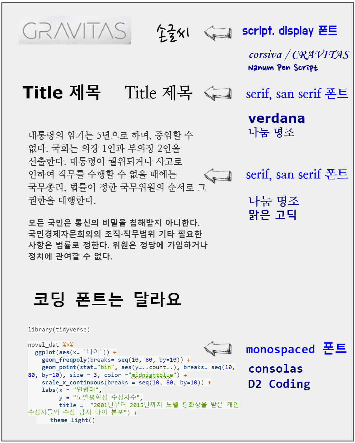
글꼴(Font)는 다양하지만 크게 다음 5가지로 영문의 경우 분류된다. 글꼴은 기본적으로 세리프(serif)와 산세리프(sans serif)의 2가지 스타일로 구분되는데 세리프는 글자의 획 끝에 작은 삐침이 있는 글꼴이며 산스(sans)은 라틴어로 없다는 뜻이기 때문에 삐침이 없는 글꼴을 지칭합니다.

serif
sans serif
script
monospaced
display

가장 쉽게 분류되는 monospaced 글꼴은 코드를 작성하기 위해 등간격을 갖는 글꼴로 consolas, D2 Coding이 대표적이다. 산세리프(Sans serif)와 세리프(Serif) 글꼴은 본문에 사용하기 적합하지만, 좀더 시선을 끄는 디자인을 위해서는 조금 더 매력적인 디스플레이(Display) 혹은 스크립트(Script)을 선택하고, 제목(Title)에는 산세리프 글꼴을 사용하는 것이 일반적이다.

1.1 `typeface` vs `font`

typeface는 서체로 번역되고 font는 글꼴로 번역된다. 하나의 typeface에 다수 font가 포함될 수 있다. 팬그램(Pangram)은 ’모든 글자’라는 뜻으로 주어진 모든 문자를 적어도 한 번 이상 사용하여 만든 문장을 뜻한다. 팬그램은 로렘 입숨처럼 글꼴 샘플을 보여주거나 장비를 테스트하는 데 사용된다. 영어 팬그램으로 가장 유명한 ’The quick brown fox jumps over the lazy dog’는 19세기부터 사용되어 왔다.

1.2 문서 - R 마크다운

아래 서체(typeface, font family)는 Noto Sans CJK KR이나 글꼴(font)은 크기, 굵기, 스타일에 따라 다양하게 텍스트를 표현할 수 있다.

서체(typeface, Noto Sans CJK KR)

다람쥐 헌 쳇바퀴에 타고파

글꼴(font)

다람쥐 헌 쳇바퀴에 타고파

R마크다운에서 다양한 서체를 글꼴을 달리하여 표현하는 방식은 css를 해당 텍스트에 다음과 같이 적용하는 것이다.

<p style="font-family: Noto Sans CJK KR; font-size:17pt; font-style:italic, font-weight:200">
다람쥐 헌 쳇바퀴에 타고파
</p>

2 글꼴 출력²

fontface에 대한 감을 갖기 위해 대표 글꼴을 ggplot으로 화면에 찍어본다.

library(tidyverse)

fonttable <- tribble(~"Short", ~"Canonical",
                         "mono", "Courier",
                         "sans", "Helvetica",
                         "serif", "Times",
                         "", "AvantGarde",
                         "", "Bookman",
                         "", "Helvetica-Narrow",
                         "", "NewCenturySchoolbook",
                         "", "Palatino",
                         "", "URWGothic",
                         "", "URWBookman",
                         "", "NimbusMon",
                         "URWHelvetica", "NimbusSan",
                         "", "NimbusSanCond",
                         "", "CenturySch",
                         "", "URWPalladio",
                         "URWTimes", "NimbusRom")

fonttable <- fonttable %>% 
  mutate(pos = row_number())

fonttable_tbl <- fonttable %>% 
  pivot_longer(cols = c(Short, Canonical), names_to = "NameType", values_to = "Font")

# Face table
facetable <- tibble ("Face" = c("plain","bold","italic","bold.italic")) %>% 
  mutate(Face = factor(Face, levels = c("plain","bold","italic","bold.italic")))

fullfonts <- merge(fonttable_tbl, facetable)

fullfonts %>% 
  ggplot(aes(x=NameType, y=pos)) +
    geom_text(aes(label=Font, family=Font, fontface=Face)) +
  facet_wrap(~ Face, ncol=2)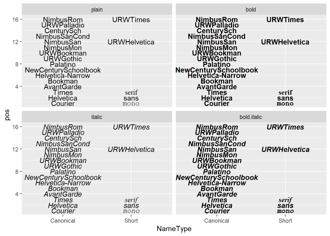

3 R 글꼴

ggplot에 텍스트를 화면에 표현하는 그래픽 장치(Graphics Device, GD)는 5가지가 존재한다.

png()
pdf()
스크린 화면 : Windows
스크린 화면 : Mac
스크린 화면 : Linux

5가지 그래픽 장치는 서로 달라 정확한 텍스트를 화면이나 png, pdf 파일이나 이미지에 넣는 것은 쉽지 않지만, 다음 팩키지가 그 역할을 수행하고 있다.

showtext
extrafont
systemfonts

4 `font` 문제지

ggplot 그래프에 담아내야 하는 글꼴은 다양한 것이 포함된다. 코드에 대한 글꼴(consolas, D2 Coding 등), 이모지 글꼴, 한글/영문 글꼴 등 다양한다.

4.1 환경설정

로고, 이모지, 코딩에 해당되는 글꼴을 R에서 불러와서 사용할 수 있도록 준비한다. .ttf 트루타입 폰트 대신 .otf 폰트를 설치할 수 있는 showtext 팩키지를 폰트 관리자(?)로 사용한다.

library(tidyverse)
library(ragg)
library(systemfonts)
library(showtext)

## 로고 
font_add("Font Awesome 5 brands",
         regular = "Font Awesome 5 Free-Regular-400.otf")

## 코딩 - Consolas, D2 Coding
font_add("Consolas",
         regular    = "consola.ttf",
         bold       = "consolab.ttf",
         italic     = "consolai.ttf",
         bolditalic = "consolaz.ttf")

font_add("D2 Coding",
         regular    = "D2Coding-Ver1.3.2-20180524.ttf",
         bold       = "D2CodingBold-Ver1.3.2-20180524.ttf")

## 이모지 폰트
font_add("Twitter Color Emoji",
         regular    = "TwitterColorEmoji-SVGinOT.ttf")
# font_add("Noto Color Emoji",
#          regular    = "NotoColorEmoji.ttf")

font_families()

[1] "sans"                  "serif"                 "mono"                 
[4] "wqy-microhei"          "Font Awesome 5 brands" "Consolas"             
[7] "D2 Coding"             "Twitter Color Emoji"

4.2 영문 테스트

“The quick brown fox jumps over the lazy dog” 영문 텍스트와 관련하여 영어로 생길 수 있는 다양한 사례를 바탕으로 글꼴을 ggplot에 찍어보자.

## 예제 텍스트 

code <- "x <- y != z : Consolas"
logo <- "twitter : Font Awesome 5 brands"
fallback_text <- "This is English, 이것은 한국어다. この文は日本語です 🚀"
emojis <- "👩🏾💻🔥📊🤩🧑🦯"
english_text <- "The quick brown fox jumps over the lazy dog"


eng_p <- ggplot() + 
  geom_text(
    aes(x = 0, y = 5, label = code), 
    family = "Consolas", size = 15
  ) + 
  geom_text(
    aes(x = 0, y = 4, label = logo), 
    family = "Font Awesome 5 brands", size = 15
  ) + 
  geom_text(
    aes(x = 0, y = 3, label = fallback_text), 
    family = "serif", size = 15
  ) + 
  geom_text(
    aes(x = 0, y = 2, label = emojis), 
    family = "Twitter Color Emoji", size = 15
  ) + 
  geom_text(
    aes(x = 0, y = 1, label = english_text), 
    family = "sans", size = 15
  ) + 
  expand_limits(y = c(0, 5)) +
  theme_void()

eng_p %>% 
  ggsave(filename = "fig/ggplot-tyopgraphy-eng.png")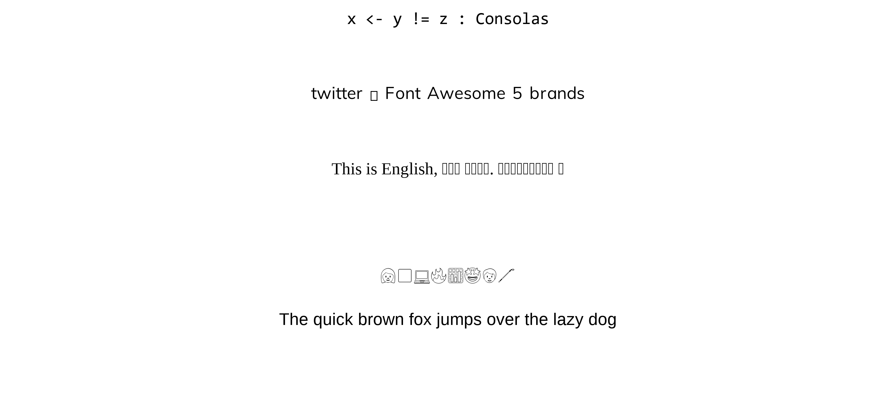

4.3 한글 테스트

## 예제 텍스트 
korean_text <- "다람쥐 헌 쳇바퀴에 타고파: Noto Sans CJK KR"
korean_code <- "library(tidyvere); x <- y != z; #한글 주석 : D2 Coding"
logo <- "twitter"
emojis <- "👩🏾💻🔥📊🤩🧑🦯"
fallback_text <- "This is English, 이것은 한국어다. この文は日本語です 🚀: Noto Sans CJK KR"

# 시각화
kor_p <- ggplot() + 
  geom_text(
    aes(x = 0, y = 5, label = korean_text), 
    family = "Noto Sans CJK KR", size = 15
  ) + 
  geom_text(
    aes(x = 0, y = 4, label = korean_code), 
    family = "D2 Coding", size = 15
  ) + 
  geom_text(
    aes(x = 0, y = 3, label = logo), 
    family = "Font Awesome 5 brands", size = 15
  ) + 
  geom_text(
    aes(x = 0, y = 2, label = emojis), 
    family = "Twitter Color Emoji", size = 15
  ) + 
  geom_text(
    aes(x = 0, y = 1, label = fallback_text), 
    family = "Noto Sans CJK KR", size = 15
  ) + 
  expand_limits(y = c(0, 5)) +
  theme_void()

kor_p %>% 
  ggsave(filename = "fig/ggplot-tyopgraphy.png")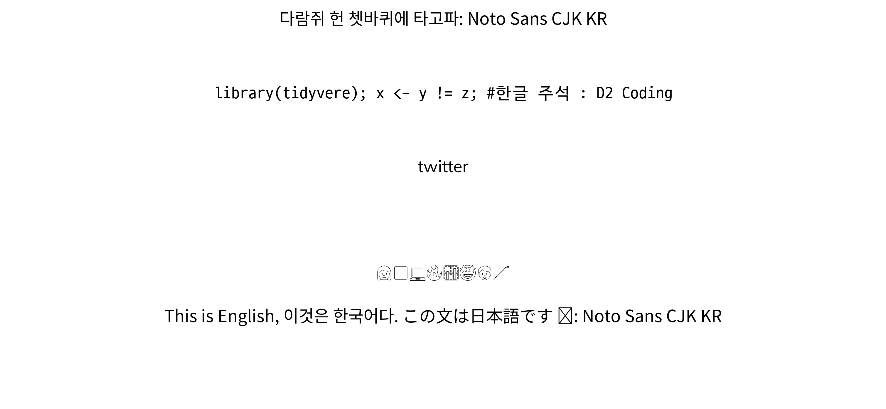

데이터 과학자 이광춘 저작

kwangchun.lee.7@gmail.com

PDF를 데이터로 보는 올바른 자세

글꼴(font)

이광춘

2021-02-27

1 글꼴 분류¹

1.1 `typeface` vs `font`

1.2 문서 - R 마크다운

2 글꼴 출력²

3 R 글꼴

4 `font` 문제지

4.1 환경설정

4.2 영문 테스트

4.3 한글 테스트

PDF를 데이터로 보는 올바른 자세

글꼴(font)

이광춘

2021-02-27

1 글꼴 분류1

1.1 typeface vs font

1.2 문서 - R 마크다운

2 글꼴 출력2

3 R 글꼴

4 font 문제지

4.1 환경설정

4.2 영문 테스트

4.3 한글 테스트

1 글꼴 분류¹

1.1 `typeface` vs `font`

2 글꼴 출력²

4 `font` 문제지