트위터 감성 예측
데이터셋
캐글웹사이트 Twitter sentiment analysis 경쟁 웹사이트에서 트위터 감성분석 데이터를 다운로드 받는다.
작업흐름도
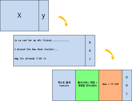
트위터 감성 예측을 위해서 $X$ 와 $y$를 확실히 구분하는 예측모형이 필요하고 $X$가 트위터와 같은 텍스트라도 이를 숫자로 변환시켜 예측모형을 구축하는 것이 가능하다. 특히 예측모형의 성능은 예측모형 자체로도 의미가 성능을 높일 수 있지만 그보다도 Feature를 발굴하여 넣어주는 것이 경우에 따라서 더 좋은 성능에 영향을 준다고 알려져 있다.
데이터 가져오기
가장 먼저 트위터 웹사이트에서 다운로드 받은 감성분류 데이터를 판다스로 불러온다.
UnicodeDecodeError when reading CSV file in Pandas with Python오류인코딩이 문제라
read_csv()메쏘드에encoding = "ISO-8859-1"을 넣어주거나,encoding = "utf-8"을 넣어주면 문제가 많이 해결된다. https://stackoverflow.com/questions/18171739/unicodedecodeerror-when-reading-csv-file-in-pandas-with-python
데이터가 여러 사람의 노력으로 라벨(label)이 Sentiment 변수에 0 혹은 1로 코딩되어 있고 데이터 사전에는 다음과 같이 데이터셋을 설명하고 있다.
- ItemID - id of twit
- Sentiment - sentiment
- 0 : negative
- 1 : positive
- SentimentText - text of the twit
import pandas as pd

df = pd.read_csv("data/twitter_sentiment_train.csv", encoding = "ISO-8859-1")
df.columns = ["item_id", "sentiment", "text"]
df.head()
# 1. 문자갯수
df['char_cnt'] = df['text'].apply(len)

# 2. 단어갯수
def count_words(text):
    '''
        문장을 입력받아 단어갯수를 반환한다.
    '''
    words = text.split()
    return len(words)

df['word_cnt'] = df['text'].apply(count_words)

# 3. 해쉬태그(#) 갯수
def count_hashtag(text):
    '''
        문장을 입력받아 해쉬태그(#)를 센다
    '''
    words = text.split()

    hashtags = [word for word in words if word.startswith('#')]
    return len(hashtags)

df['hashtag_cnt'] = df['text'].apply(count_hashtag)

# 4. 언급(@) 갯수
def count_mention(text):
    '''
        문장을 입력받아 언급횟수(@)를 센다
    '''
    words = text.split()

    mentions = [word for word in words if word.startswith('@')]
    return len(mentions)

df['mention_cnt'] = df['text'].apply(count_mention)


df.tail()
트위터 트윗에서 내장된 len 함수와 count_mention, count_hashtag, count_words와 같은 사용자 정의 함수를 통해서 기초적인 텍스트 Feature를 추출해냈다. 이를 바탕으로 감성분류기 성능이 어느 정도 나오는지 예측 모형을 생성해보자.
나이브 베이즈 예측모형을 훈련/시험 데이터로 분리하고 이를 적합시켜 나온 예측모형 정확도를 통해 기준모형으로 삼아도 좋을 듯 싶다.
# 나이브 베이즈 모형
from sklearn.naive_bayes import MultinomialNB
from sklearn.model_selection import train_test_split

# 훈련/시험 데이터 분리
string_df = df[['char_cnt', 'word_cnt', 'hashtag_cnt', 'mention_cnt']]

target = df['sentiment']

X_train, X_test, y_train, y_test  = train_test_split(string_df, target, test_size=0.3)

# 예측모형 적합
clf = MultinomialNB()

# Fit the classifier
clf.fit(X_train, y_train)

# Measure the accuracy
accuracy = clf.score(X_test, y_test)
print("시험 데이터셋으로 검정한 감성 분류 예측모형 정확도: %.3f" % accuracy)
읽기 점수(readability score)
영어문장에 대해 읽기 점수(readability score) 측정하여 이를 Feature로 넣어 예측모형 정확도를 높여나간다. 이를 위해서 Flesch–Kincaid readability tests 사례를 들면 다음 공식에 의해서 읽기 점수가 부여된다.
$$206.835 - 1.015 \left( \frac{\text{total words}}{\text{total sentences}} \right) - 84.6 \left( \frac{\text{total syllables}}{\text{total words}} \right)$$| 점수 | 학년 | 설명 | |
|---|---|---|---|
| 100-90 | 5학년 | 읽기 쉽고, 11살 학생도 쉽게 이해함 | |
| 90–80 | 6학년 | 읽기 쉽고, 고객을 위한 대화형태 영어 | |
| 80–70 | 중1(7th grade) | 상당히 읽기 쉬움 | |
| 70–60 | 중2,3(8th & 9th grade) | 평이한 영문, 13 ~ 15세 학생도 쉽게 이해함 | students. |
| 60–50 | 고등학생 | 나름 읽기 어려움 | |
| 50–30 | 대학생 | 읽기 어려움 | |
| 30–0 | 대학원생 | 매우 읽기 어려움, 대학원생은 잘 이해함 |
읽기 점수 계산을 위해서 textatistic 라이브러리가 필요한데 다음 명령어를 쉘에서 입력하게 되면 수월하게 설치할 수 있다.
$ pip install textatistic
stackoverflow를 참조하여 영화 리뷰데이터를 가져와서 읽기 점수를 산출해본다. textatistic 0.0.1을 참조하면 다양한 읽기점수 통계량을 확인할 수 있다.
dalechall_score: Dale-Chall score.flesch_score: Flesch Reading Ease score.fleschkincaid_score: Flesch-Kincaid score.gunningfog_score: Gunning Fog score.smog_score: SMOG score.
import pandas as pd
from nltk.corpus import movie_reviews as mr
from textatistic import Textatistic

# 읽기점수 산출 함수
def calc_readability(text):
    readability_scores = Textatistic(text).scores
    score = readability_scores['fleschkincaid_score']
    return score

# 영화 리뷰 데이터
reviews = []

for file_id in mr.fileids():
    tag, filename = file_id.split('/')
    reviews.append((filename, tag, mr.raw(file_id)))

movie_df = pd.DataFrame(reviews, columns=['filename', 'tag', 'text'])

movie_df.head()
sample_movie_df = movie_df.sample(n=10)

sample_movie_df['fleschkincaid_score'] = sample_movie_df['text'].apply(calc_readability)
sample_movie_df.head()