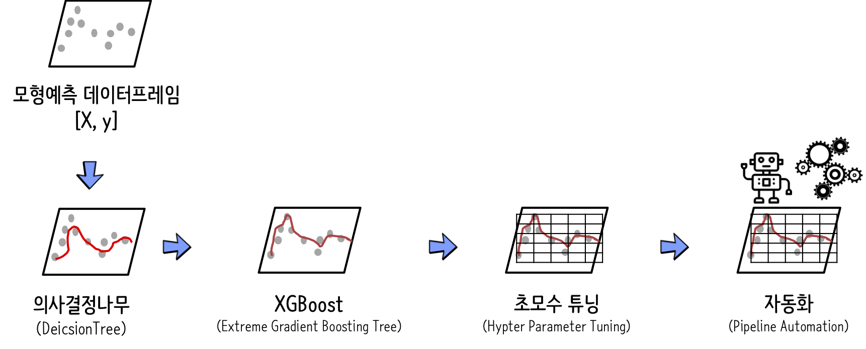
XGBoost 예측모형 자동화

XGBoost 예측모형은 뛰어난 성능으로 이미 캐글 등 대다수 경진대회를 휩쓴 검증된 알고리즘이다. 그렇다고 모든 예측문제에 기계학습 알고리즘으로 선택을 할 수는 없다. 우선, 뛰어난 성능을 가진 XGBoost 알고리즘의 마지막까지 높일 수 있는 초모수(Hyper Paramter) 튜닝에 대해서 살펴보자. Tianqi Chen (Oct. 22 2014), "Introduction to Boosted Trees", Washington University

XGBoost

초모수(Hypter parameter) 튜닝

XGBoost와 관련된 Hypter Parameter는 다음 세가지 범주로 나뉜다. XGBoost가 의사결정나무에 기반하기 때문에 관련된 모수와 기계학습과 관련이 있기 때문에 이와 연관된 다수 초모수가 포함된다.

  • 학습 초모수
    • objective [기본설정값=reg:linear]: 지도학습 손실 최소화 함수를 정의
      • binary:logistic: 이항 분류 문제 로직스틱 회귀모형으로 반환값이 클래스가 아니라 예측 확률.
      • multi:softmax: 다항 분류 문제의 경우 소프트맥스(Softmax)를 사용해서 분류하는데 반횐되는 값이 예측확률이 아니라 클래스임. 또한 num_class도 지정해야함.
      • multi:softprob: 각 클래스 범주에 속하는 예측확률을 반환함.
    • eval_metric: 설정한 objective별로 기본설정값이 지정되어 있음.
      • rmse: root mean square error
      • mae: mean absolute error
      • logloss: negative log-likelihood
      • error: Binary classification error rate (0.5 threshold)
      • merror: Multiclass classification error rate
      • mlogloss: Multiclass logloss
      • auc: Area under the curve
    • seed [기본설정값: 0]: 재현가능하도록 난수를 고정시킴.
  • 일반 초모수
    • booster: 의사결정 기반 모형(gbtree), 선형 모형(linear)
    • mthread: 병렬처리에 사용되는 코어수, 특정값을 지정하지 않는 경우 자동으로 시스템 코어수를 탐지하여 병렬처리에 동원함.
  • 부스팅 초모수
    • eta [기본설정값: 0.3]: GBM에 학습율과 유사하고 일반적으로 0.01 ~ 0.2 값이 사용됨
    • min_child_weight [기본설정값: 1]: 과적합(overfitting)을 방지할 목적으로 사용되는데, 너무 높은 값은 과소적합(underfitting)을 야기하기 때문에 CV를 사용해서 적절한 값이 제시되어야 한다.
    • max_depth [기본설정값: 6]: 과적합 방지를 위해서 사용되는데 역시 CV를 사용해서 적절한 값이 제시되어야 하고 보통 3-10 사이 값이 적용된다.
    • max_leaf_nodes: max_leaf_nodes 값이 설정되면 max_depth는 무시된다. 따라서 두값 중 하나를 사용한다.
    • max_delta_step [기본설정값: 0]: 일반적으로 잘 사용되지 않음.
    • subsample [기본설정값: 1]: 개별 의사결정나무 모형에 사용되는 임의 표본수를 지정. 보통 0.5 ~ 1 사용됨.
    • colsample_bytree [기본설정값: 1]: 개별 의사결정나무 모형에 사용될 변수갯수를 지정. 보통 0.5 ~ 1 사용됨.
    • colsample_bylevel [기본설정값: 1]: subsample, colsample_bytree 두 초모수 설정을 통해서 이미 의사결정나무 모형 개발에 사용될 변수갯수와 관측점 갯수를 사용했는데 추가로 colsample_bylevel을 지정하는 것이 특별한 의미를 갖는지 의문이 듦.
    • lambda [기본설정값: 1]: 능선 회쉬(Ridge Regression)의 L2 정규화(regularization) 초모수. 그다지 많이 사용되고 있지는 않음.
    • alpha [기본설정값: 0]: 라쏘 회귀(Lasso Regression)의 L1 정규화(regularization) 초모수로 차원이 높은 경우 알고리즘 속도를 높일 수 있음.
    • scale_pos_weight [기본설정값: 1]: 클래스 불균형이 심한 경우 0보다 큰 값을 지정하여 효과를 볼 수 있음.

참고문헌: Analytics Vidhya, "Complete Guide to Parameter Tuning in XGBoost with codes in Python"

XGBoost 초모수

XGBoost 초모수(Hyper Parameter)는 XGBoost 객체를 하나 생성한 후에 print() 함수로 확인이 가능하다. 그렇다고 모든 Hyper parameter가 중요한 것은 아니다.

In [1]:
import xgboost as xgb

xgb_clf = xgb.XGBClassifier()

print(xgb_clf)
XGBClassifier(base_score=0.5, booster='gbtree', colsample_bylevel=1,
              colsample_bynode=1, colsample_bytree=1, gamma=0,
              learning_rate=0.1, max_delta_step=0, max_depth=3,
              min_child_weight=1, missing=None, n_estimators=100, n_jobs=1,
              nthread=None, objective='binary:logistic', random_state=0,
              reg_alpha=0, reg_lambda=1, scale_pos_weight=1, seed=None,
              silent=None, subsample=1, verbosity=1)

XGBoost 초모수 헬로월드

XGBoost 초모수를 간단한 헬로월드 코드를 작성해본다.

In [2]:
# 경고 출력하지 않음 -----------
import warnings
warnings.filterwarnings('ignore')

# 라이브러리와 데이터 가져오기
import numpy as np
import pandas as pd
from sklearn.model_selection import train_test_split
import xgboost as xgb
import sklearn
from sklearn.metrics import classification_report, accuracy_score

print('sklearn version: %s' % sklearn.__version__)
print('xgboost version: %s' % xgb.__version__)

hr_df = pd.read_csv("data/HR_comma_sep.csv")
hr_df.head()

# 시험/훈련 데이터 관측점 구분
colnames = ['satisfaction_level', 'last_evaluation', 'number_project', 'average_montly_hours', 'time_spend_company', 'Work_accident', 
       'promotion_last_5years']

X, y = hr_df[colnames], hr_df[['left']]
X_train, X_test, y_train, y_test= train_test_split(X, y, test_size=0.3, random_state=777)

# XGBoost 예측모형
xgb_model = xgb.XGBClassifier(silent=False, 
                              booster='gbtree',
                              scale_pos_weight=1,
                              learning_rate=0.01,  
                              colsample_bytree = 0.4,
                              subsample = 0.8,
                              objective='binary:logistic', 
                              n_estimators=100, 
                              max_depth=4, 
                              gamma=10, 
                              seed=777)

hr_pred = xgb_model.fit(X_train, y_train).predict(X_test)
print(classification_report(y_test, hr_pred))
sklearn version: 0.21.2
xgboost version: 0.90
              precision    recall  f1-score   support

           0       0.91      1.00      0.95      3440
           1       0.99      0.68      0.80      1060

    accuracy                           0.92      4500
   macro avg       0.95      0.84      0.88      4500
weighted avg       0.93      0.92      0.92      4500

초모수 1개 대상 예측모형 구축

max_depth 의사결정나무 모형 깊이 초모수를 달리해서 XGBoost 예측모형의 성능을 비교해본다.

In [3]:
accuracy_list = []

max_depth_list = [3,5,7,9,10]

for max_depth in max_depth_list:
    xgb_model = xgb.XGBClassifier(max_depth=max_depth, seed=777)
    xgb_pred = xgb_model.fit(X_train, y_train).predict(X_test)
    xgb_accuracy = accuracy_score(y_test, xgb_pred) 
    accuracy_list.append(xgb_accuracy)
    
xgb_df = pd.DataFrame({'tree depth':max_depth_list, 'accuracy':accuracy_list})
xgb_df.head()    
Out[3]:
tree depth accuracy
0 3 0.974889
1 5 0.979333
2 7 0.982222
3 9 0.983556
4 10 0.984889

교차검증(CV, Cross-Validation)

강건한 예측모형 구축을 위해서 훈련데이터를 교차검증(Cross-Validation)을 통해서 과적합을 방지시킬 수 있는 모형을 구축할 수 있다. 즉 훈련데이터를 3조각, 5조각 혹은 10조각을 내서 1조각을 제외한 나머지 조각을 훈련에 사용하고 모형성능을 1조각으로 평가시켜 가장 강건한 모형을 예측모형으로 선정한다.

In [4]:
hr_dmatrix = xgb.DMatrix(data=hr_df[colnames], label=hr_df[['left']])

cv_params = {"objective":"binary:logistic", 
             "n_estimators": 100, 
             "max_depth":5}

hr_cv = xgb.cv(dtrain=hr_dmatrix, 
               params=cv_params, 
               nfold=5, 
               num_boost_round=10, 
               metrics="auc", 
               as_pandas=True)

hr_cv
Out[4]:
train-auc-mean train-auc-std test-auc-mean test-auc-std
0 0.976151 0.000584 0.974546 0.004580
1 0.980073 0.001645 0.977836 0.003115
2 0.982462 0.000626 0.980670 0.002991
3 0.982992 0.000624 0.981325 0.002830
4 0.984424 0.001160 0.982618 0.002191
5 0.985397 0.000821 0.983066 0.002788
6 0.986158 0.000351 0.984041 0.002888
7 0.987001 0.000325 0.984812 0.002570
8 0.987493 0.000397 0.985092 0.002536
9 0.987849 0.000569 0.985406 0.002380

시각화

XGBoost 모형을 시각화함으로써 개발한 예측모형의 성능에 대해 더 깊은 이해를 가질 수 있다. xgb.plot_importance() 메쏘드에 XGBoost 모형객체를 넣어 변수중요도를 파악할 수 있다. 특히 의사결정나무 시각화를 위해서 graphviz 라이브러리 설치가 필요한데... 경로명 설정문제도 함께 해결하는 방식으로 아래와 같이 pip install, conda install 명령어를 연이어 실행시킨다.

  • pip install graphviz
  • conda install graphviz

참고자료: frhyme.code, "graphviz 다시 설치하기"

In [5]:
xgb.plot_importance(xgb_model)
Out[5]:
<matplotlib.axes._subplots.AxesSubplot at 0x1a1e051690>
In [6]:
xgb.plot_tree(xgb_model, num_trees=3)
Out[6]:
<matplotlib.axes._subplots.AxesSubplot at 0x1a1e2035d0>
In [7]:
xgb.to_graphviz(xgb_model, num_trees=3)
Out[7]:
%3 0 satisfaction_level<0.465000004 1 number_project<3 0->1 yes, missing 2 time_spend_company<5 0->2 no 3 last_evaluation<0.574999988 1->3 yes, missing 4 satisfaction_level<0.114999995 1->4 no 5 average_montly_hours<291 2->5 yes, missing 6 last_evaluation<0.814999998 2->6 no 7 last_evaluation<0.444999993 3->7 yes, missing 8 average_montly_hours<278 3->8 no 9 leaf=0.156779587 4->9 yes, missing 10 number_project<7 4->10 no 15 leaf=-0.140828729 7->15 yes, missing 16 average_montly_hours<164 7->16 no 17 leaf=-0.140699729 8->17 yes, missing 18 leaf=0.0196444262 8->18 no 27 average_montly_hours<126 16->27 yes, missing 28 satisfaction_level<0.295000017 16->28 no 43 leaf=-0.120573714 27->43 yes, missing 44 satisfaction_level<0.340000004 27->44 no 45 leaf=0.0449607037 28->45 yes, missing 46 leaf=-0.126797736 28->46 no 67 leaf=-0.0528328419 44->67 yes, missing 68 leaf=0.155873537 44->68 no 19 average_montly_hours<289 10->19 yes, missing 20 leaf=0.12497177 10->20 no 29 last_evaluation<0.995000005 19->29 yes, missing 30 leaf=0.114781462 19->30 no 47 satisfaction_level<0.305000007 29->47 yes, missing 48 satisfaction_level<0.194999993 29->48 no 69 satisfaction_level<0.145000011 47->69 yes, missing 70 satisfaction_level<0.335000008 47->70 no 71 leaf=0.0449607037 48->71 yes, missing 72 leaf=-0.0949949846 48->72 no 87 time_spend_company<3 69->87 yes, missing 88 leaf=-0.150756001 69->88 no 89 number_project<5 70->89 yes, missing 90 last_evaluation<0.965000033 70->90 no 99 number_project<5 87->99 yes, missing 100 Work_accident<1 87->100 no 109 leaf=-0.0411673337 99->109 yes, missing 110 leaf=0.0966307893 99->110 no 111 leaf=-0.140711769 100->111 yes, missing 112 leaf=-0.0703829974 100->112 no 101 leaf=-0.119641535 89->101 yes, missing 102 time_spend_company<5 89->102 no 103 leaf=-0.140895814 90->103 yes, missing 104 leaf=-0.00800376292 90->104 no 113 leaf=-0.0475379825 102->113 yes, missing 114 leaf=0.116312467 102->114 no 11 number_project<6 5->11 yes, missing 12 leaf=0.106788218 5->12 no 13 last_evaluation<0.805000007 6->13 yes, missing 14 average_montly_hours<217 6->14 no 21 satisfaction_level<0.474999994 11->21 yes, missing 22 last_evaluation<0.965000033 11->22 no 31 average_montly_hours<209 21->31 yes, missing 32 leaf=-0.153790861 21->32 no 33 average_montly_hours<163 22->33 yes, missing 34 satisfaction_level<0.75999999 22->34 no 49 leaf=-0.128160313 31->49 yes, missing 50 leaf=0.0295562986 31->50 no 51 average_montly_hours<155 33->51 yes, missing 52 satisfaction_level<0.644999981 33->52 no 53 leaf=0.0217539892 34->53 yes, missing 54 leaf=-0.0588356145 34->54 no 73 leaf=-0.127582461 51->73 yes, missing 74 leaf=0.120179094 51->74 no 75 average_montly_hours<249 52->75 yes, missing 76 leaf=-0.15104875 52->76 no 91 leaf=-0.0897278935 75->91 yes, missing 92 leaf=0.00394297903 75->92 no 23 average_montly_hours<273 13->23 yes, missing 24 time_spend_company<6 13->24 no 25 last_evaluation<0.975000024 14->25 yes, missing 26 time_spend_company<7 14->26 no 35 time_spend_company<6 23->35 yes, missing 36 satisfaction_level<0.574999988 23->36 no 37 satisfaction_level<0.75999999 24->37 yes, missing 38 leaf=-0.106788218 24->38 no 55 average_montly_hours<243 35->55 yes, missing 56 leaf=-0.155474588 35->56 no 57 last_evaluation<0.659999967 36->57 yes, missing 58 leaf=-0.126318797 36->58 no 77 leaf=-0.134132728 55->77 yes, missing 78 satisfaction_level<0.774999976 55->78 no 93 leaf=-0.118065335 78->93 yes, missing 94 satisfaction_level<0.805000007 78->94 no 105 leaf=0.108343318 94->105 yes, missing 106 leaf=-0.104150392 94->106 no 79 leaf=0.019743178 57->79 yes, missing 80 leaf=-0.0306103975 57->80 no 59 leaf=-0.0208277609 37->59 yes, missing 60 leaf=0.0471658967 37->60 no 39 number_project<3 25->39 yes, missing 40 satisfaction_level<0.774999976 25->40 no 41 satisfaction_level<0.704999983 26->41 yes, missing 42 leaf=-0.147899449 26->42 no 61 leaf=-0.0544177853 39->61 yes, missing 62 leaf=-0.144523412 39->62 no 63 leaf=0.0170837063 40->63 yes, missing 64 last_evaluation<0.985000014 40->64 no 81 leaf=-0.00819887128 64->81 yes, missing 82 leaf=-0.096236594 64->82 no 65 last_evaluation<0.915000021 41->65 yes, missing 66 number_project<4 41->66 no 83 leaf=-0.118996553 65->83 yes, missing 84 average_montly_hours<248 65->84 no 85 leaf=-0.109490655 66->85 yes, missing 86 number_project<6 66->86 no 95 leaf=-0.0493735485 84->95 yes, missing 96 leaf=0.0327930488 84->96 no 97 satisfaction_level<0.915000021 86->97 yes, missing 98 leaf=-0.0669936165 86->98 no 107 leaf=0.151778981 97->107 yes, missing 108 number_project<5 97->108 no 115 leaf=-0.00390869332 108->115 yes, missing 116 leaf=0.116105832 108->116 no

3가지 초모수 튜닝

일반적으로 초모수(Hypter Parameter)를 튜닝하는 방식은 격자 탐색(Grid Search), 임의 탐색(Random Search), 베이즈 최적화(Bayesian Optimization) 방식이 많이 사용된다. 가장 기본적인 격자 탐색을 이해하고 이를 바탕으로 실무에서는 베이즈 최적화를 사용하도록 하자.

for 루프를 사용한 튜닝

모수가 하나 혹은 두개인 경우 for 루플 사용해서 최적 초모수를 결정할 수 있다.

In [8]:
hr_accuracy_list = []

max_depth_list = [1,3,5,7,9]

def hr_grid_search(max_depth): 
    xgb_model = xgb.XGBClassifier(max_depth=max_depth)
    xgb_pred = xgb_model.fit(X_train, y_train).predict(X_test)
    
    return([max_depth, accuracy_score(y_test, xgb_pred)])
      

for max_depth in max_depth_list:
    hr_accuracy_list.append(hr_grid_search(max_depth))

    
hr_xgb_df = pd.DataFrame(hr_accuracy_list, columns=['tree depth', 'accuracy'])
hr_xgb_df.head()    
Out[8]:
tree depth accuracy
0 1 0.910000
1 3 0.974889
2 5 0.979333
3 7 0.982222
4 9 0.983556

탐색할 초모수 숫자가 늘어나게 되면 for 루프를 계속해서 중첩시켜야 한다. 이는 가독성도 떨어뜨리고 추후 유지보수에 상당한 문제를 야기시킨다.

In [9]:
hr2_accuracy_list = []

max_depth_list = [3,5,7]
subsample_list = [0.6, 0.8, 1.0]

def hr2_grid_search(max_depth, subsample): 
    xgb_model = xgb.XGBClassifier(max_depth=max_depth,
                              subsample=subsample)
    xgb_pred = xgb_model.fit(X_train, y_train).predict(X_test)
    
    return([max_depth, subsample, accuracy_score(y_test, xgb_pred)])
      

for max_depth in max_depth_list:
    for subsample in subsample_list:
        hr2_accuracy_list.append(hr2_grid_search(max_depth, subsample))
    
hr2_xgb_df = pd.DataFrame(hr2_accuracy_list, columns=['tree depth', 'subsample rate', 'accuracy'])
hr2_xgb_df.head() 
Out[9]:
tree depth subsample rate accuracy
0 3 0.6 0.974667
1 3 0.8 0.975111
2 3 1.0 0.974889
3 5 0.6 0.978667
4 5 0.8 0.979333

격자 탐색(Grid Search)

for 문을 대신하여 격자 탐색(Grid Search)를 사용해서 깔끔하게 코드를 정리해보자. 먼저 분류모형(estimator)를 XGBoost로 지정하고 XGBoost 모형의 초모수를 딕셔너리로 지정하여 초모수 격자를 생성시킨다.

In [10]:
from sklearn.model_selection import GridSearchCV

# XGBoost 분류기 생성
xgb_clf = xgb.XGBClassifier()

# 초모수 격자생성
xgb_param_grid = {'max_depth': [3,5,7], 
              'subsample': [0.6, 0.8, 1.0]}

# Create a GridSearchCV object
hr_grid = GridSearchCV(estimator=xgb_clf,
                       param_grid=xgb_param_grid,
                       scoring='roc_auc',
                       n_jobs=8,
                       cv=5,
                       refit=True, 
                       return_train_score=True)

hr_grid.fit(X_train, y_train)
Out[10]:
GridSearchCV(cv=5, error_score='raise-deprecating',
             estimator=XGBClassifier(base_score=0.5, booster='gbtree',
                                     colsample_bylevel=1, colsample_bynode=1,
                                     colsample_bytree=1, gamma=0,
                                     learning_rate=0.1, max_delta_step=0,
                                     max_depth=3, min_child_weight=1,
                                     missing=None, n_estimators=100, n_jobs=1,
                                     nthread=None, objective='binary:logistic',
                                     random_state=0, reg_alpha=0, reg_lambda=1,
                                     scale_pos_weight=1, seed=None, silent=None,
                                     subsample=1, verbosity=1),
             iid='warn', n_jobs=8,
             param_grid={'max_depth': [3, 5, 7], 'subsample': [0.6, 0.8, 1.0]},
             pre_dispatch='2*n_jobs', refit=True, return_train_score=True,
             scoring='roc_auc', verbose=0)

격자 탐색이 완료되면 이를 데이터프레임으로 바꾸어서 모수에 대한 사항을 살펴보고 최적 초모수를 감별한다.

In [11]:
hr_grid_df = pd.DataFrame(hr_grid.cv_results_)
hr_grid_df.loc[:, ['mean_test_score', "params"]]
Out[11]:
mean_test_score params
0 0.987299 {'max_depth': 3, 'subsample': 0.6}
1 0.987182 {'max_depth': 3, 'subsample': 0.8}
2 0.987056 {'max_depth': 3, 'subsample': 1.0}
3 0.991230 {'max_depth': 5, 'subsample': 0.6}
4 0.991056 {'max_depth': 5, 'subsample': 0.8}
5 0.990975 {'max_depth': 5, 'subsample': 1.0}
6 0.991625 {'max_depth': 7, 'subsample': 0.6}
7 0.991856 {'max_depth': 7, 'subsample': 0.8}
8 0.992205 {'max_depth': 7, 'subsample': 1.0}
In [12]:
hr_grid_df[hr_grid_df['rank_test_score'] == 1]
Out[12]:
mean_fit_time std_fit_time mean_score_time std_score_time param_max_depth param_subsample params split0_test_score split1_test_score split2_test_score ... mean_test_score std_test_score rank_test_score split0_train_score split1_train_score split2_train_score split3_train_score split4_train_score mean_train_score std_train_score
8 1.209971 0.021592 0.016729 0.000867 7 1 {'max_depth': 7, 'subsample': 1.0} 0.993105 0.988505 0.991156 ... 0.992205 0.003073 1 0.998429 0.99838 0.998318 0.998676 0.997867 0.998334 0.000263

1 rows × 22 columns

격자탐색으로 나온 산출물을 정리해보자.

In [13]:
## 최고성능
best_score = hr_grid.best_score_
# 최고성능을 내는 행을 찾아냄
best_row = hr_grid.best_index_

# 최적 초모수: max_depth, subsample
best_max_depth     = hr_grid.best_params_["max_depth"]
best_max_subsample = hr_grid.best_params_["subsample"]

nl = '\n'
print(f'예측모형성능(AUC):  \t {best_score:.3f}{nl}\
        인덱스:           \t {best_row}{nl}\
        max_depth:      \t {max_depth}{nl}\
        subsample:      \t {subsample}')
예측모형성능(AUC):  	 0.992
        인덱스:           	 8
        max_depth:      	 7
        subsample:      	 1.0

임의 탐색(Random Search)

임의 탐색(Random Search)은 격자탐색과 여러가지로 유사성이 있으나 임의 추출하는 초모수 탐색횟수를 지정한다는 면에서 차이가 난다.

In [14]:
from sklearn.model_selection import RandomizedSearchCV

# XGBoost 분류기 생성
xgb_clf = xgb.XGBClassifier()

# 초모수 격자생성
xgb_param_grid = {'max_depth': list(range(2,10)), 
                  'subsample': np.linspace(0.4, 1, 7)}

# Create a random search object
xgb_random = RandomizedSearchCV(estimator = xgb_clf,
                                param_distributions = xgb_param_grid,
                                n_iter = 10,
                                scoring='roc_auc', 
                                n_jobs=8, 
                                cv = 3, 
                                refit=True, 
                                return_train_score = True)

# Fit to the training data
xgb_random.fit(X_train, y_train)
Out[14]:
RandomizedSearchCV(cv=3, error_score='raise-deprecating',
                   estimator=XGBClassifier(base_score=0.5, booster='gbtree',
                                           colsample_bylevel=1,
                                           colsample_bynode=1,
                                           colsample_bytree=1, gamma=0,
                                           learning_rate=0.1, max_delta_step=0,
                                           max_depth=3, min_child_weight=1,
                                           missing=None, n_estimators=100,
                                           n_jobs=1, nthread=None,
                                           objective='binary:logistic',
                                           random_state=0, reg_alpha=0,
                                           reg_lambda=1, scale_pos_weight=1,
                                           seed=None, silent=None, subsample=1,
                                           verbosity=1),
                   iid='warn', n_iter=10, n_jobs=8,
                   param_distributions={'max_depth': [2, 3, 4, 5, 6, 7, 8, 9],
                                        'subsample': array([0.4, 0.5, 0.6, 0.7, 0.8, 0.9, 1. ])},
                   pre_dispatch='2*n_jobs', random_state=None, refit=True,
                   return_train_score=True, scoring='roc_auc', verbose=0)
In [15]:
hr_random_df = pd.DataFrame(xgb_random.cv_results_)
hr_random_df.loc[:, ['mean_test_score', "params"]]
Out[15]:
mean_test_score params
0 0.989352 {'subsample': 0.7, 'max_depth': 4}
1 0.988768 {'subsample': 0.5, 'max_depth': 4}
2 0.990513 {'subsample': 0.8, 'max_depth': 9}
3 0.989637 {'subsample': 0.8, 'max_depth': 4}
4 0.990581 {'subsample': 0.8, 'max_depth': 7}
5 0.991309 {'subsample': 0.8999999999999999, 'max_depth': 8}
6 0.989285 {'subsample': 0.4, 'max_depth': 6}
7 0.991109 {'subsample': 0.8999999999999999, 'max_depth': 7}
8 0.990271 {'subsample': 0.7, 'max_depth': 6}
9 0.986689 {'subsample': 0.7, 'max_depth': 3}

임의 탐색 기본기(날코딩)

임의 탐색(Random Search)를 scikit-learn 라이브러리를 사용해서 RandomizedSearchCV 클래스를 동원해서 구현했다. 하지만, 격자탐색 for 루프와 마찬가지로 소위 말해서 날코딩으로 구현하는 것도 가능하다.

  1. 탐색하고자 하는 초모수 리스트를 정의한다: max_depth, subsample
  2. product 함수로 조합한 리스트를 list comprehension으로 구현한다: 이를 위해서 itertools 라이브러리 product를 사용한다.
  3. np.random.choice() 함수로 초모수 조합에서 추출한다.
  4. 이를 주어진 탐색횟수만큼 for 문을 돌려 예측모형 성능을 데이터화한다.
In [16]:
from itertools import product

# 초모수 정의: max_depth, subsample
max_depth_list = list(range(3,10))
subsample_list = np.linspace(0.1, 1, 10)

# 초모수 조합 리스트 생성
combi_list = [list(x) for x in product(max_depth_list, subsample_list)]

# 초모수 조합에서 난수 추출
random_combi_index = np.random.choice(range(1, len(combi_list)+1), 10, replace=False)
combi_random_selected = [combi_list[x] for x in random_combi_index]

# 난수로 뽑은 조합 출력
print(combi_random_selected)
[[7, 0.8], [4, 0.4], [8, 0.4], [6, 0.6], [4, 0.9], [8, 0.1], [5, 1.0], [6, 0.4], [5, 0.7000000000000001], [4, 0.2]]
In [17]:
hr_random_list = []
# 예측함수 XGBoost 정의
def hr_random_search(max_depth, subsample): 
    xgb_model = xgb.XGBClassifier(max_depth=max_depth,
                              subsample=subsample)
    xgb_pred = xgb_model.fit(X_train, y_train).predict(X_test)
    
    return([max_depth, subsample, accuracy_score(y_test, xgb_pred)])
      

for i, param in enumerate(combi_random_selected):
    hr_random_list.append(hr_random_search(param[0], param[1]))

    
hr_xgb_random_df = pd.DataFrame(hr_random_list, columns=['tree depth', 'subsample rate', 'accuracy'])
hr_xgb_random_df
Out[17]:
tree depth subsample rate accuracy
0 7 0.8 0.982222
1 4 0.4 0.976667
2 8 0.4 0.981556
3 6 0.6 0.980889
4 4 0.9 0.976889
5 8 0.1 0.973333
6 5 1.0 0.979333
7 6 0.4 0.978889
8 5 0.7 0.978667
9 4 0.2 0.974667

베이즈 최적화

Hyperopt: Distributed Asynchronous Hyper-parameter Optimization 웹사이트에서 개발버전을 다운로드 받는 것도 가능하고, !pip install hyperopt 명령어를 통해서 베이지안 최적화 라이브러리를 설치한다.

참고: District Data Labs (Dec 24, 2017), "Parameter Tuning with Hyperopt"

In [18]:
from hyperopt import fmin, tpe, hp
from sklearn.model_selection import cross_val_score

# 초모수 탐색공간 정의
param_space = {'max_depth': hp.quniform('max_depth', 2, 10, 1),
               'subsample': hp.uniform('subsample', 0.1, 0.9)}

# 목적함수 정의
def objective(params):
    params = {'max_depth': int(params['max_depth']),
              'subsample': params['subsample']}
    xgb_clf = xgb.XGBClassifier(n_estimators=100, **params) 
    best_score = cross_val_score(xgb_clf, X_train, y_train, 
                                 scoring='accuracy', 
                                 cv=5, 
                                 n_jobs=8).mean()
    loss = 1 - best_score
    return loss

# 알고리즘 실행
best = fmin(fn=objective, space=param_space, 
            max_evals=10, 
            rstate=np.random.RandomState(777), 
            algo=tpe.suggest)
print(best)
100%|██████████| 10/10 [00:09<00:00,  1.04it/s, best loss: 0.01581120386605428]
{'max_depth': 9.0, 'subsample': 0.6383870484708831}

상기 코드를 이해가 전에 먼저 간단한 예제를 통해서 베이즈 최적화기법에 대한 이해를 넓혀가자. $y=(x-1)^2$ 함수에 대한 최소값을 찾아내는 문제를 베이즈 최적화를 통해 살펴보자. 먼저 fmin() 함수에 fn에 $y=(x-1)^2$ 함수를 지정한다. 그리고 나서 검색공간에 hp.uniform()을 지정하면 베이즈 최적화를 통해 최소값을 찾아낼 수 있다.

In [19]:
best = fmin(
    fn=lambda x: (x-1)**2,
    space=hp.uniform('x', -2, 4),
    algo=tpe.suggest,
    max_evals=100)

print(best)
100%|██████████| 100/100 [00:00<00:00, 608.04it/s, best loss: 5.558957429663535e-06]
{'x': 1.0023577441399913}

상기 내용을 matplotlib으로 시각화하면 다음과 같다.

In [20]:
import matplotlib.pyplot as plt
import numpy as np

x = np.array(np.linspace(-2,4,100))
y = (x-1) ** 2

plt.plot(x,y)
plt.plot(best['x'], 0, 'ro')
plt.show()

초모수 시각화

초모수 값에 따라 예측모형의 성능변화를 시각화하는 것은 초모수 탐색공간을 줄일 수 있을 뿐만 아니라 최적 초모수 탐색에 큰 도움을 준다.

In [21]:
%matplotlib inline 
plt.rc('font', family='NanumGothicOTF') # 한글 폰트깨짐 해결(맥) 윈도우는 NanumGothic

plt.scatter(y=hr_xgb_random_df.accuracy, x=hr_xgb_random_df['tree depth'])  
plt.gca().set(xlabel='나무깊이', ylabel='정확도', title='초모수 정확도 시각화')
plt.show()